Free Throw Bias in the NBA

Disgruntled twitter heads are constantly clamoring that NBA officiating is in dire straits, their team of choice the victim of an endless league-wide conspiracy. At the bottom of the fanatics’ paranoia, there does appear to be something of a consensus that there’s such a thing as ‘superstar’ calls, i.e., a pattern of superstar players getting favorable calls that players on two-way contracts aren’t getting. This naturally leads us to ask whether there’s a bias favoring big-market teams in the association? I’ll apply some basic econometric techniques, including Bayesian posterior analytical derivation, to test the hypothesis that there is a bias in favor of big-market teams.

Let’s start by comparing the distributions of teams’ free throw attempts (FTAs) differential, denoted by $\theta$–$\theta_{it} > 0$ indicating that team $t$ attempted more free throws than their opponent in game $i$ and $\theta_{it}< 0$ indicating that team $t$ attempted fewer free throws than their opponent in game $i$. The graph below compares the distributions of FTA differences for the 2023-2024 NBA season among only the top 10 teams by average free throw differential. 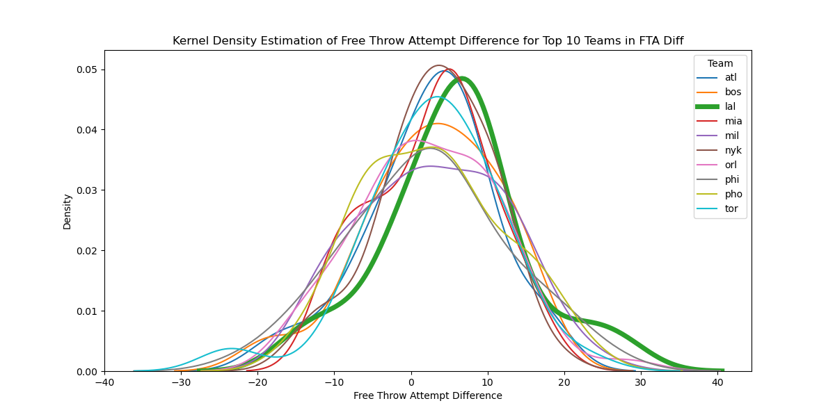Clearly, some teams get more free throws than others; using FTA difference means that we have controlled for game-specific effects, such as who the officials are or whether a game is particularly physical or soft. Nonetheless, this approach doesn’t take into account team-specific effects. In particular, note the thickness of the Los Angeles Lakers’ (in bold green) distribution’s right tail.

This information is, at most, merely suggestive: after all, teams can play a certain way to earn more or fewer free throws. For example, they can be more physically dominant in the paint (where shooting fouls are likelier to occur) or they could more frequently settle for jump shots (less likely to draw shooting fouls). Looking at the distributions above, there might be differences in play style that are driving the variation in FTA difference; therefore, let’s control for some indicators of style of play. Employing the same dataset as above, I next ran a mulitple linear OLS regression, with the $\theta_{it}$ as the dependent variable, following the specification below (for game $i$ and team $t$):

In the equation above, $\mu_t$ is the team fixed-effects term, captured by a set of dummy variables for every single team. Thus, the coefficients attached to these dummy variables may be interpreted as estimates for $\mu_t$. I’ve plotted those estimates below: 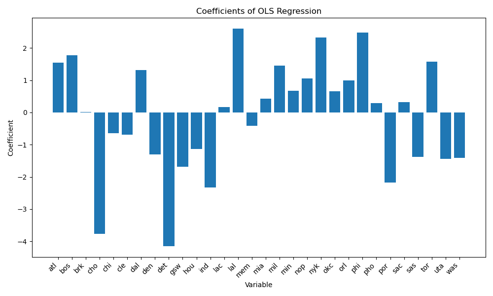Three teams get the largest ‘bonus’, other factors being controlled for: the Los Angeles Lakers, the New York Knicks, and the Philadelphia 76ers. Unsurprisingly, these are three big-market teams and marquee franchises–the Knicks are the 2nd-most valuable NBA franchise, the Lakers the 3rd, and the Sixers the 9th, as of December 2023.

Let’s conclude by using Bayesian methods to derive the posterior curve for each of these teams; these curves suggest possible estimates of the ‘true’ value of a team’s free throw attempts. We combine the knowledge granted to us by our priors–in this case, the total distribution of free throw difference–with the real distribution of observations for team $t$ to plot the conditional probability of $\theta$. Because of the nature of the free throw difference data, I fit it to a normal curve: 1) free throw difference will always be centered on 0 (for a complete dataset of teams and games), 2) free throw differences closer to 0 are much likelier than free throw differences away from 0, and 3) free throw difference will follow a unimodal (rather than bimodal, for example) distribution. Here I’ve ploted the total distribution, the fitted normal curve, and the means for my three teams of interest: 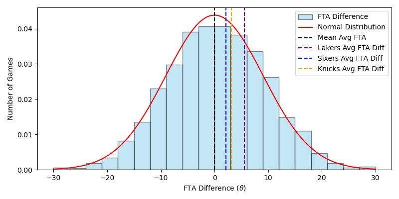The fitted normal curve represents my prior information about the distribution of free throw attempt differences. Next, I estimate the posterior curve yielded by Bayes’ Theorem:

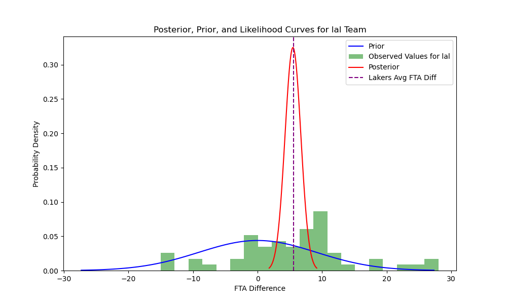
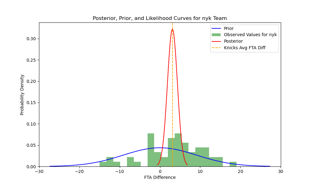
Where $\theta$ is our outcome of interest–the free throw attempt difference for a particular team. Next, I use the normal likelihood estimator to find the resultant posteriors for the Lakers, Knicks, and Sixers. 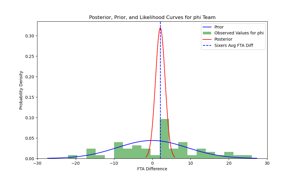These curves re-affirm that the Lakers, Knicks, and Sixers all receive a much greater advantage in free throw attempts than the rest of the league, and the distribution of their observed values dominates the prior (hence the steepness of the posterior curves). Another way to visualize the posterior curves is to sample repeatedly from them and to plot the distributions for these samples. Thus, I sample from the posterior 5,000 times to create the following histograms: 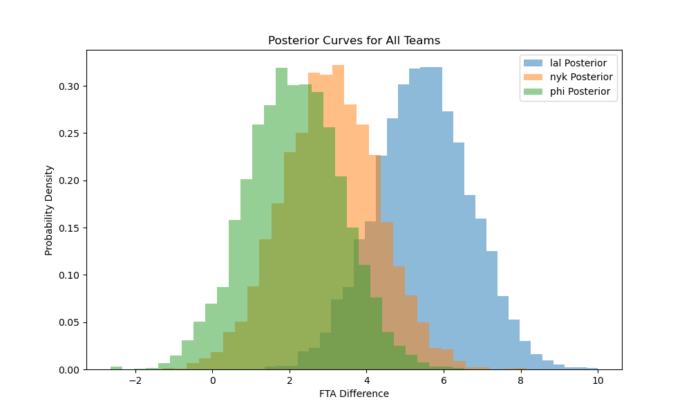Clearly, the Lakers’ distribution of free throw attempt differences skews more heavily to the right than the Knicks of Sixers, although all three teams’ posteriors are centered significantly to the right of 0, the center of the prior distribution.

Next, using the posteriors crafted above, we can conduct further analysis, including finding the posterior probability or Bayesian confidence intervals. For this analysis, let’s focus on the Lakers, who appear to receive the most significant advantage in free throw attempts.

Let’s begin with the posterior probability that $\theta_{\text{lal}} > 0$, since 0 is the center of the league’s total distribution of $\theta$. The probability, as we might expect from the graphs above, is 100%. What about a $\theta$ greater than one standard deviation of the prior above 0? The probability of that is merely 0.12%, and the probability of $\theta$ being greater than two standard deviations above 0 is 0%. Finally, the posterior probability that the Lakers shoot more free throws than the Knicks’ mean is 96.84% and for the Sixers’ mean is 99.78%. Now let’s compute a Bayesian confidence interval; at a 90% confidence level, the interval is (3.50,7.48) and at 95%, the interval is (3.06,7.85). Clearly, we can say with a great deal of confidence that the Lakers have a greater free throw attempt advantage than the rest of the league.

This approach suggests that there is some obvious advantage for big-market teams, in particular for the Lakers, Knicks, and Sixers. However, there are some shortcomings: the team data I’ve used for my analysis includes only the most basic information about shooting patterns–in fact, it only tells me whether a field goal attempt was a 2-pointer or a 3-pointer. And although in my regression analysis above, I included rebounds as a proxy for a team’s physical domination of the paint, that’s an imperfect measure. Ideally, I would be able to control for the distribution of 2-point field attempts by distance from the basket–the assumption being that shoots within 0-3 feet of the basketball are much likelier to draw fouls than shoots attempted 16 feet from the basket. Unfortunately, that data is only available for individual players.

To address these shortcomings, in a future blog post I’ll hone in on individual players; if I look at individual players’ careers who played for the Lakers as well as other NBA teams, I can control for more detailed variables like shooting patterns (specifically the distance from the basket of their average 2 point field attempt), individual honors won, age, and winning percentage in games played in an attempt to isolate a possible ‘Los Angeles Premium’ for free throw attempts. I will also derive the posterior curves for selected current Los Angeles players (most importantly Lebron James and Anthony Davis), using their past seasons’ free throw attempt data as the prior information and their free throw attempts while in a Lakers uniform as the parameter of interest.

Data is taken from Basketball Reference.

Code and Data